Supervised Image Denosing with MSDNets and SMSNet ensembles

Authors: Eric Roberts and Petrus Zwart

E-mail: PHZwart@lbl.gov, EJRoberts@lbl.gov

This notebook highlights some basic functionality with the dlsia package.

In this notebook we setup a Mixed-Scaled Dense Network (MSDNet) and train it to denoising image corrupted by Gaussian noise. Subsequently, we will train a number Randomized Sparse Networks (RMSNets) on the same task and show how to obtain error estimates via ensemble methods.

import sys
import os
import numpy as np
import tqdm

import torch
import torch.nn as nn
import torch.optim as optim

import matplotlib.pyplot as plt
from torch.utils.data import DataLoader, Dataset

import h5py
from torchsummary import summary

from dlsia.core import helpers
from dlsia.core.train_scripts import train_regression
from dlsia.core.networks import msdnet, smsnet, baggins
from dlsia.test_data.two_d import build_test_data, torch_hdf5_loader
from dlsia.viz_tools import plots, draw_sparse_network

import matplotlib.pyplot as plt

Create Data

We produce noisy, single-class data consisting of peaks in guassian noise. This data will be generated using hdf5 files .

Parameters to toggle:

• batch_size : number of images passed through GPU at a single time

• n_imgs : number of images in training set

• n_peaks : number of circular peaks in each image

• n_xy : size of images

• snr : signal-to-noise ratio; more noise for lower number

makeData = True
batch_size = 100
num_workers = 0
showNoisyData = True
use_scaled_data = True

Generate hdf5 peak data

if makeData == True:
    n_imgs = 200
    n_peaks = 8
    n_xy = 32
    snr=3
    mask_radius = 1.0

    build_test_data.build_data_standard_sets_2d(n_imgs=n_imgs,
                                                n_peaks=n_peaks,
                                                n_xy=n_xy,
                                                snr=snr,
                                                mask_radius=mask_radius)

100%|████████████████████████████████████████████████████████████| 20/20 [00:00<00:00, 269.52it/s]
100%|████████████████████████████████████████████████████████████| 10/10 [00:00<00:00, 465.98it/s]
100%|███████████████████████████████████████████████████████████████| 1/1 [00:00<00:00, 60.96it/s]

Load hdf5 peak data

Data generator class above can generate the following:

• trax_GT : ground truth

• trax_obs : obstructed, noisy images

• trax_obs_norm : noisy images linearly scaled to interal [0,1]

• trax_mask : binary masked images indicating peak (1) or background (0)

if use_scaled_data == True:
    x_label = "trax_obs_norm"
else:
    x_label = "trax_obs"

f_train = "train_data_2d.hdf5"
f_test  = "test_data_2d.hdf5"
f_validation = "validate_data_2d.hdf5"

MyData_train = torch_hdf5_loader.Hdf5Dataset2D(filename=f_train,
                                               x_label=x_label,
                                               y_label="trax_GT")
MyData_validation = torch_hdf5_loader.Hdf5Dataset2D(filename=f_validation,
                                                    x_label=x_label,
                                                    y_label="trax_GT")
MyData_test = torch_hdf5_loader.Hdf5Dataset2D(filename=f_test,
                                              x_label=x_label,
                                              y_label="trax_GT")

loader_params = {'batch_size': batch_size, 'shuffle': True, 'num_workers': num_workers}
train_loader = DataLoader(MyData_train, **loader_params)
loader_params = {'batch_size': batch_size, 'shuffle': False, 'num_workers': num_workers}
validation_loader = DataLoader(MyData_validation, **loader_params)
test_loader = DataLoader(MyData_test, **loader_params)

View peak data

if showNoisyData == True:
    for batch in train_loader:
        noisy, mask = batch

        plt.figure(figsize=(12,10))
        plt.subplot(321)
        plt.imshow(noisy[0,0,:,:]); plt.colorbar(shrink=0.8); plt.title('Noisy');
        plt.subplot(322);
        plt.imshow(mask[0,0,:,:]); plt.colorbar(shrink=0.8); plt.title('Mask');
        plt.subplot(323)
        plt.imshow(noisy[1,0,:,:]); plt.colorbar(shrink=0.8)
        plt.subplot(324);
        plt.imshow(mask[1,0,:,:]); plt.colorbar(shrink=0.8)
        plt.subplot(325)
        plt.imshow(noisy[2,0,:,:]); plt.colorbar(shrink=0.8)
        plt.subplot(326);
        plt.imshow(mask[2,0,:,:]); plt.colorbar(shrink=0.8)

        break

    plt.rcParams.update({'font.size': 18})
    plt.tight_layout()
    plt.show()

Create and train MSDNet

Lots of options to customize. See dlsia/core/networks/msdnet.py

in_channels = 1
out_channels = 1
num_layers = 40
max_dilation = 8
activation = nn.ReLU()
normalization = nn.BatchNorm2d

msdnet_model = msdnet.MixedScaleDenseNetwork(in_channels = in_channels,
                                             out_channels = out_channels,
                                             num_layers=num_layers,
                                             max_dilation = max_dilation,
                                             activation=activation,
                                             normalization=normalization,
                                            )

pytorch_total_params = sum(p.numel() for p in msdnet_model.parameters() if p.requires_grad)
print("Total number of refineable parameters: ", pytorch_total_params)

Total number of refineable parameters:  9182

Train the model

We perform the following:

• specify number of epochs,

• select the L2 MSE loss as our scroing criteria,

• select a learning rate of 1/1000

• choose the popular Adam optimizer for traversing the loss terrain

epochs = 100   # set number of epochs
criterion = nn.MSELoss()
learning_rate = 1e-2

optimizer = optim.Adam(msdnet_model.parameters(), lr=learning_rate)

device = helpers.get_device()
msdnet_model.to(device)
msdnet_model, results = train_regression(msdnet_model,
                                         train_loader,
                                         validation_loader,
                                         epochs,
                                         criterion,
                                         optimizer,
                                         device=device,
                                         show=10
                                        )
torch.cuda.empty_cache()

Epoch 10 of 100 | Learning rate 1.000e-02
Training Loss: 2.0480e-02 | Validation Loss: 1.9214e-02
Training CC: 0.6652   Validation CC  : 0.6940
Epoch 20 of 100 | Learning rate 1.000e-02
Training Loss: 9.7999e-03 | Validation Loss: 9.5666e-03
Training CC: 0.8558   Validation CC  : 0.8613
Epoch 30 of 100 | Learning rate 1.000e-02
Training Loss: 7.6222e-03 | Validation Loss: 7.7206e-03
Training CC: 0.8899   Validation CC  : 0.8896
Epoch 40 of 100 | Learning rate 1.000e-02
Training Loss: 6.4154e-03 | Validation Loss: 6.6536e-03
Training CC: 0.9082   Validation CC  : 0.9057
Epoch 50 of 100 | Learning rate 1.000e-02
Training Loss: 5.4005e-03 | Validation Loss: 5.6188e-03
Training CC: 0.9232   Validation CC  : 0.9210
Epoch 60 of 100 | Learning rate 1.000e-02
Training Loss: 4.6870e-03 | Validation Loss: 4.9463e-03
Training CC: 0.9338   Validation CC  : 0.9308
Epoch 70 of 100 | Learning rate 1.000e-02
Training Loss: 4.3836e-03 | Validation Loss: 4.5876e-03
Training CC: 0.9383   Validation CC  : 0.9360
Epoch 80 of 100 | Learning rate 1.000e-02
Training Loss: 4.0819e-03 | Validation Loss: 4.4152e-03
Training CC: 0.9426   Validation CC  : 0.9385
Epoch 90 of 100 | Learning rate 1.000e-02
Training Loss: 3.9863e-03 | Validation Loss: 4.3827e-03
Training CC: 0.9440   Validation CC  : 0.9390
Epoch 100 of 100 | Learning rate 1.000e-02
Training Loss: 3.9378e-03 | Validation Loss: 4.3817e-03
Training CC: 0.9447   Validation CC  : 0.9390

plots.plot_training_results_regression(results)

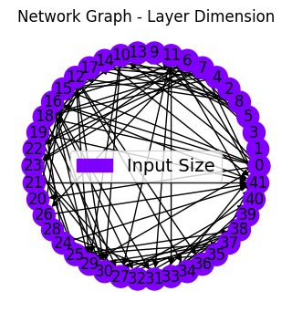
Create and train SMSNets

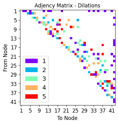
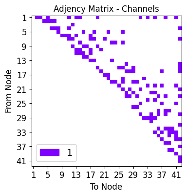
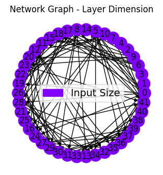
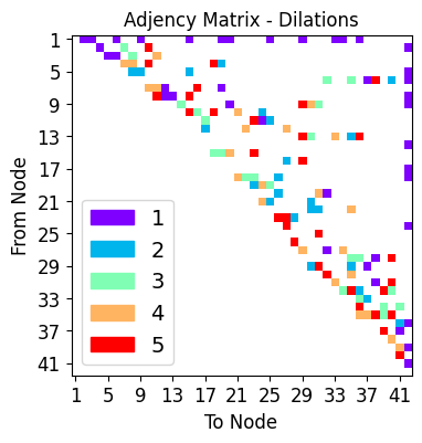
Sparse versions of MSDNets with randomly connected layers and dilations are created here

Specify hyperparameters

Next, the hyperparameters below govern the random network connectivity. Choices include:

• alpha : modifies distribution of consecutive connection length between network layers/nodes,

• gamma : modifies distribution of of layer/node degree,

• IL : probability of connection between Input node and Layer node,

• IO : probability of connection between Input node and Output node,

• LO : probability of connection between Layer node and Output node,

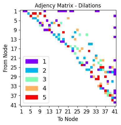
• dilation_choices : set of possible dilations along each individual node connection

The specific parameters and what they do are described in detail in the documentation. Please follow minor minor comments below for a more cursory explanation.

in_channels = 1 # RGB input image
out_channels = 1 # binary output
num_layers = 40

# When alpha > 0, short-range skip connections are favoured
alpha = 0.20

# When gamma is 0, the degree of each node is chosen uniformly between 0 and max_k
# specifically, P(degree) \propto degree^-gamma
gamma = 0.0

# we can limit the maximum and minimum degree of our graph
max_k = 6
min_k = 3

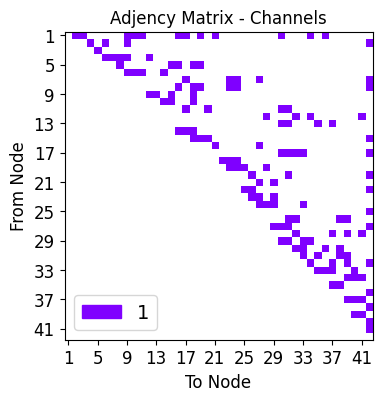
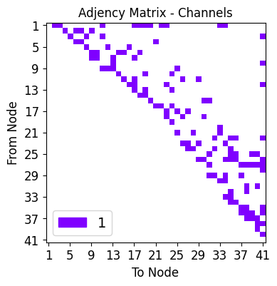
# features channel posibilities per edge
hidden_out_channels = [1]

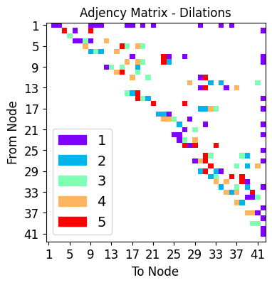
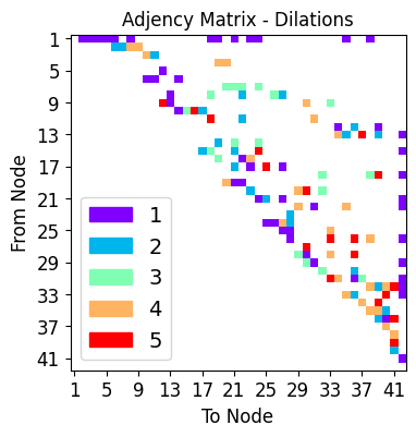
# possible dilation choices
dilation_choices = [1,2,3,4,5]

# Here are some parameters that define how networks are drawn at random
# the layer probabilities dictionairy define connections
layer_probabilities={'LL_alpha':alpha,
                     'LL_gamma': gamma,
                     'LL_max_degree':max_k,
                     'LL_min_degree':min_k,
                     'IL': 0.25,
                     'LO': 0.25,
                     'IO': False}

# if desired, one can introduce scale changes (down and upsample)
# a not-so-thorough look indicates that this isn't really super beneficial
# in the model systems we looked at
sizing_settings = {'stride_base':2, #better keep this at 2
                   'min_power': 0,
                   'max_power': 0}

# defines the type of network we want to build

network_type = "Regression"

Build networks and train

We specify the number of random networks to initialize and the number of epochs for each is trained.

nets = []
n_networks = 7
epochs = 50     # Set number of epochs
criterion = nn.MSELoss()   # For segmenting
learning_rate = 1e-2

for ii in range(n_networks):
    torch.cuda.empty_cache()
    print("Network %i"%(ii+1))
    smsnet_model = smsnet.random_SMS_network(in_channels=in_channels,
                                             out_channels=out_channels,
                                             in_shape=(32,32),
                                             out_shape=(32,32),
                                             sizing_settings=sizing_settings,
                                             layers=num_layers,
                                             dilation_choices=dilation_choices,
                                             hidden_out_channels=hidden_out_channels,
                                             layer_probabilities=layer_probabilities,
                                             network_type=network_type
                                            )

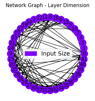
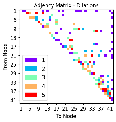
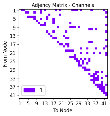
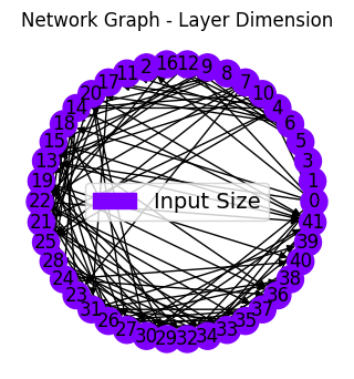
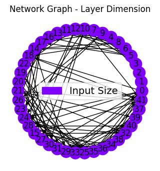
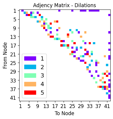
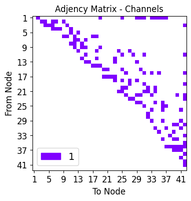
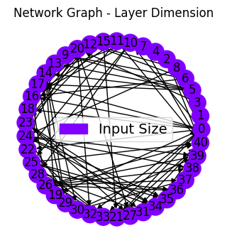
    # lets plot the network
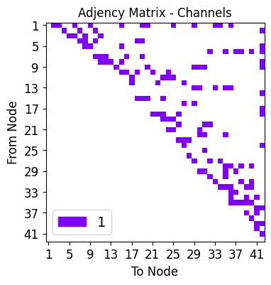
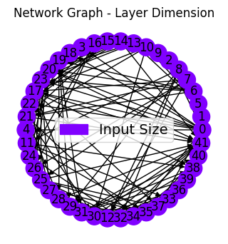
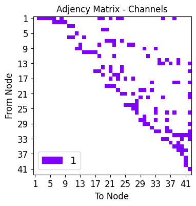
    net_plot,dil_plot,chan_plot = draw_sparse_network.draw_network(smsnet_model)
    plt.show()

    nets.append(smsnet_model)

    print("Start training")
    pytorch_total_params = sum(p.numel() for p in smsnet_model.parameters() if p.requires_grad)
    print("Total number of refineable parameters: ", pytorch_total_params)

    optimizer = optim.Adam(smsnet_model.parameters(), lr=learning_rate)  # Defined in loop, one per network
    device = helpers.get_device()
    smsnet_model = smsnet_model.to(device)
    tmp = train_regression(smsnet_model,
                           train_loader,
                           test_loader,
                           epochs,
                           criterion,
                           optimizer,
                           device,
                           show=10)
    smsnet_model = smsnet_model.cpu()
    plots.plot_training_results_regression(tmp[1]).show()

Network 1

Start training
Total number of refineable parameters:  3939
Epoch 10 of 50 | Learning rate 1.000e-02
Training Loss: 9.2175e-03 | Validation Loss: 8.0032e-03
Training CC: 0.8686   Validation CC  : 0.8800
Epoch 20 of 50 | Learning rate 1.000e-02
Training Loss: 6.0803e-03 | Validation Loss: 6.5273e-03
Training CC: 0.9140   Validation CC  : 0.9042
Epoch 30 of 50 | Learning rate 1.000e-02
Training Loss: 5.1456e-03 | Validation Loss: 5.8442e-03
Training CC: 0.9271   Validation CC  : 0.9151
Epoch 40 of 50 | Learning rate 1.000e-02
Training Loss: 4.6548e-03 | Validation Loss: 5.4656e-03
Training CC: 0.9343   Validation CC  : 0.9213
Epoch 50 of 50 | Learning rate 1.000e-02
Training Loss: 4.3191e-03 | Validation Loss: 5.2219e-03
Training CC: 0.9392   Validation CC  : 0.9249

Network 2

Start training
Total number of refineable parameters:  3990
Epoch 10 of 50 | Learning rate 1.000e-02
Training Loss: 9.1804e-03 | Validation Loss: 8.0699e-03
Training CC: 0.8771   Validation CC  : 0.8871
Epoch 20 of 50 | Learning rate 1.000e-02
Training Loss: 6.4843e-03 | Validation Loss: 6.6771e-03
Training CC: 0.9072   Validation CC  : 0.9031
Epoch 30 of 50 | Learning rate 1.000e-02
Training Loss: 5.6728e-03 | Validation Loss: 6.0229e-03
Training CC: 0.9194   Validation CC  : 0.9134
Epoch 40 of 50 | Learning rate 1.000e-02
Training Loss: 5.1018e-03 | Validation Loss: 5.5597e-03
Training CC: 0.9277   Validation CC  : 0.9200
Epoch 50 of 50 | Learning rate 1.000e-02
Training Loss: 4.6591e-03 | Validation Loss: 5.3416e-03
Training CC: 0.9344   Validation CC  : 0.9233

Network 3

Start training
Total number of refineable parameters:  3669
Epoch 10 of 50 | Learning rate 1.000e-02
Training Loss: 1.2144e-02 | Validation Loss: 1.2543e-02
Training CC: 0.8506   Validation CC  : 0.8502
Epoch 20 of 50 | Learning rate 1.000e-02
Training Loss: 6.7236e-03 | Validation Loss: 7.7115e-03
Training CC: 0.9041   Validation CC  : 0.8868
Epoch 30 of 50 | Learning rate 1.000e-02
Training Loss: 5.6058e-03 | Validation Loss: 6.9776e-03
Training CC: 0.9203   Validation CC  : 0.8990
Epoch 40 of 50 | Learning rate 1.000e-02
Training Loss: 5.0782e-03 | Validation Loss: 6.8975e-03
Training CC: 0.9282   Validation CC  : 0.9011
Epoch 50 of 50 | Learning rate 1.000e-02
Training Loss: 4.6339e-03 | Validation Loss: 6.3910e-03
Training CC: 0.9346   Validation CC  : 0.9080

Network 4

Start training
Total number of refineable parameters:  3663
Epoch 10 of 50 | Learning rate 1.000e-02
Training Loss: 1.3449e-02 | Validation Loss: 1.3231e-02
Training CC: 0.7986   Validation CC  : 0.8016
Epoch 20 of 50 | Learning rate 1.000e-02
Training Loss: 8.0801e-03 | Validation Loss: 8.5300e-03
Training CC: 0.8832   Validation CC  : 0.8727
Epoch 30 of 50 | Learning rate 1.000e-02
Training Loss: 6.4468e-03 | Validation Loss: 7.3383e-03
Training CC: 0.9077   Validation CC  : 0.8927
Epoch 40 of 50 | Learning rate 1.000e-02
Training Loss: 5.5732e-03 | Validation Loss: 6.9593e-03
Training CC: 0.9207   Validation CC  : 0.8992
Epoch 50 of 50 | Learning rate 1.000e-02
Training Loss: 4.9964e-03 | Validation Loss: 6.5431e-03
Training CC: 0.9292   Validation CC  : 0.9049

Network 5

Start training
Total number of refineable parameters:  3462
Epoch 10 of 50 | Learning rate 1.000e-02
Training Loss: 1.1155e-02 | Validation Loss: 1.0104e-02
Training CC: 0.8359   Validation CC  : 0.8501
Epoch 20 of 50 | Learning rate 1.000e-02
Training Loss: 7.0713e-03 | Validation Loss: 7.0207e-03
Training CC: 0.8985   Validation CC  : 0.8984
Epoch 30 of 50 | Learning rate 1.000e-02
Training Loss: 5.5692e-03 | Validation Loss: 5.8999e-03
Training CC: 0.9208   Validation CC  : 0.9132
Epoch 40 of 50 | Learning rate 1.000e-02
Training Loss: 4.8418e-03 | Validation Loss: 5.3266e-03
Training CC: 0.9315   Validation CC  : 0.9219
Epoch 50 of 50 | Learning rate 1.000e-02
Training Loss: 4.3537e-03 | Validation Loss: 4.8718e-03
Training CC: 0.9387   Validation CC  : 0.9287

Network 6

Start training
Total number of refineable parameters:  3619
Epoch 10 of 50 | Learning rate 1.000e-02
Training Loss: 1.2206e-02 | Validation Loss: 1.0908e-02
Training CC: 0.8169   Validation CC  : 0.8338
Epoch 20 of 50 | Learning rate 1.000e-02
Training Loss: 7.2262e-03 | Validation Loss: 7.5402e-03
Training CC: 0.8960   Validation CC  : 0.8896
Epoch 30 of 50 | Learning rate 1.000e-02
Training Loss: 5.7538e-03 | Validation Loss: 6.8879e-03
Training CC: 0.9181   Validation CC  : 0.8989
Epoch 40 of 50 | Learning rate 1.000e-02
Training Loss: 4.9582e-03 | Validation Loss: 6.1591e-03
Training CC: 0.9298   Validation CC  : 0.9098
Epoch 50 of 50 | Learning rate 1.000e-02
Training Loss: 4.5296e-03 | Validation Loss: 5.7084e-03
Training CC: 0.9362   Validation CC  : 0.9171

Network 7

Start training
Total number of refineable parameters:  3326
Epoch 10 of 50 | Learning rate 1.000e-02
Training Loss: 1.3265e-02 | Validation Loss: 1.2832e-02
Training CC: 0.8193   Validation CC  : 0.8177
Epoch 20 of 50 | Learning rate 1.000e-02
Training Loss: 6.9772e-03 | Validation Loss: 7.6696e-03
Training CC: 0.9005   Validation CC  : 0.8864
Epoch 30 of 50 | Learning rate 1.000e-02
Training Loss: 5.6950e-03 | Validation Loss: 6.9365e-03
Training CC: 0.9193   Validation CC  : 0.8983
Epoch 40 of 50 | Learning rate 1.000e-02
Training Loss: 5.0621e-03 | Validation Loss: 6.5130e-03
Training CC: 0.9284   Validation CC  : 0.9049
Epoch 50 of 50 | Learning rate 1.000e-02
Training Loss: 4.6441e-03 | Validation Loss: 6.2002e-03
Training CC: 0.9344   Validation CC  : 0.9100

Testing our models

Finally, we load testing data, pass it through the network, and save results as .png

Helper functions

def regression_metrics( preds, target):
    """
    Here, the Pearson correlation coefficient is calulated between the network
    predictions and the ground truth.
    """
    tmp = corcoef.cc(preds.cpu().flatten(), target.cpu().flatten() )
    return(tmp)


def segment_imgs(testloader, net, num_display=10, plot=True, std=False):
    """
    This function makes network predictions on testing data found in the 'testloader'
    pytorch dataloader object.

    :param testloader: the pyTorch dataloader object used to retrieve testing data
    :param net: the trained deep network
    :param plot: do you want to plot the first 10 network results using matplotlib?

    :returns seg_imgs: the predicted images, concatenated into a single tensor
    :returns noisy_imgs: the input images, concatenated into a single tensor
    :returns target_imgs: the ground truth images, concatenated into a single tensor
    """
    torch.cuda.empty_cache()

    seg_imgs = []
    noisy_imgs = []
    #target_imgs = []

    #running_CC_test_val = 0.0

    counter = 0
    with torch.no_grad():
        for batch in testloader:
            num_display = np.minimum(num_display, len(batch[0]))
            noisy, target = batch

            noisy = torch.FloatTensor(noisy)
            noisy = noisy.to(device)#.unsqueeze(1)

            sigmas = None
            if not std:
                output = net.to(device)(noisy)
            else:
                output, sigmas = net.to(device)(noisy, 'cpu', True)

            if counter == 0:
                seg_imgs = output.detach().cpu()
                noisy_imgs = noisy.detach().cpu()
                target_imgs = target.detach().cpu()
                if std:
                    sigmas = sigmas.detach().cpu()
            else:
                seg_imgs = torch.cat((seg_imgs, output.detach().cpu()), 0)
                noisy_imgs = torch.cat((noisy_imgs, noisy.detach().cpu()), 0)
                target_imgs = torch.cat((target_imgs, target.detach().cpu()), 0)
                if std:
                    sigmas = sigmas.detach().cpu()


            counter+=1

            if plot==True:
                for j in range(5):
                    if not std:
                        print(f'Images for batch # {counter}, number {j}')
                        plt.figure(figsize=(22,5))
                        plt.rcParams.update({'font.size': 20})

                        plt.subplot(131)
                        plt.imshow(noisy.cpu()[j,0,:,:].data); plt.colorbar(shrink=0.8); plt.title('Noisy');
                        plt.subplot(132)
                        plt.imshow(output[j,0,:,:].detach().cpu()); plt.colorbar(shrink=0.8); plt.title('Prediction');
                        plt.subplot(133)
                        plt.imshow(target.cpu()[j,0,:,:].data); plt.colorbar(shrink=0.8); plt.title('Ground Truth');

                        plt.tight_layout()

                        plt.show()
                    else:
                        print(f'Images for batch # {counter}, number {j}')
                        plt.figure(figsize=(22,5))
                        plt.rcParams.update({'font.size': 20})

                        plt.subplot(151)
                        plt.imshow(noisy.cpu()[j,0,:,:].data);
                        plt.colorbar(shrink=0.8); plt.title('Noisy');
                        plt.subplot(152)
                        plt.imshow(output[j,0,:,:].detach().cpu());
                        plt.colorbar(shrink=0.8); plt.title('Prediction');
                        plt.subplot(153)
                        plt.imshow(sigmas[j,0,:,:].detach().cpu());
                        plt.colorbar(shrink=0.8); plt.title('Sigmas');
                        plt.subplot(154)
                        plt.imshow(output[j,0,:,:].detach().cpu() / sigmas[j,0,:,:].detach().cpu(),vmax=30);
                        plt.colorbar(shrink=0.8); plt.title('Signal to Noise');

                        plt.subplot(155)
                        plt.imshow(target.cpu()[j,0,:,:].data); plt.colorbar(shrink=0.8); plt.title('Ground Truth');

                        plt.tight_layout()

                        plt.show()




    #CC = running_CC_test_val / len(testloader)
    torch.cuda.empty_cache()
    return seg_imgs, noisy_imgs, target_imgs

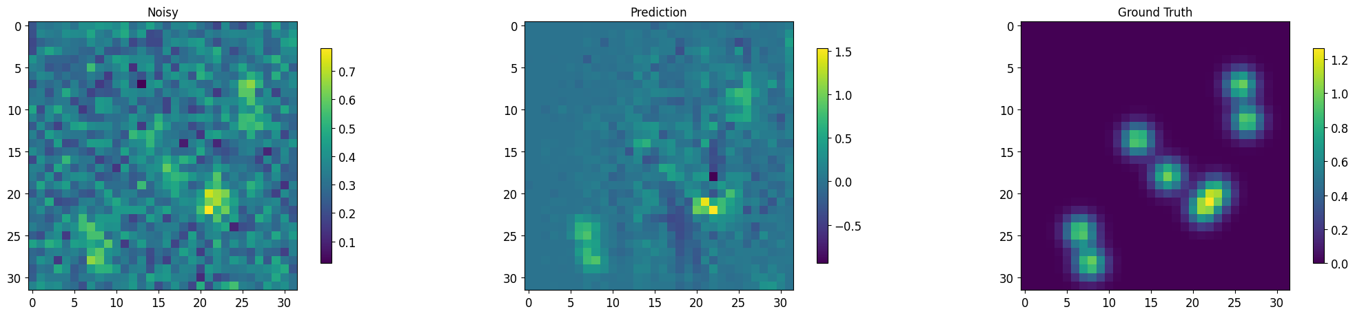
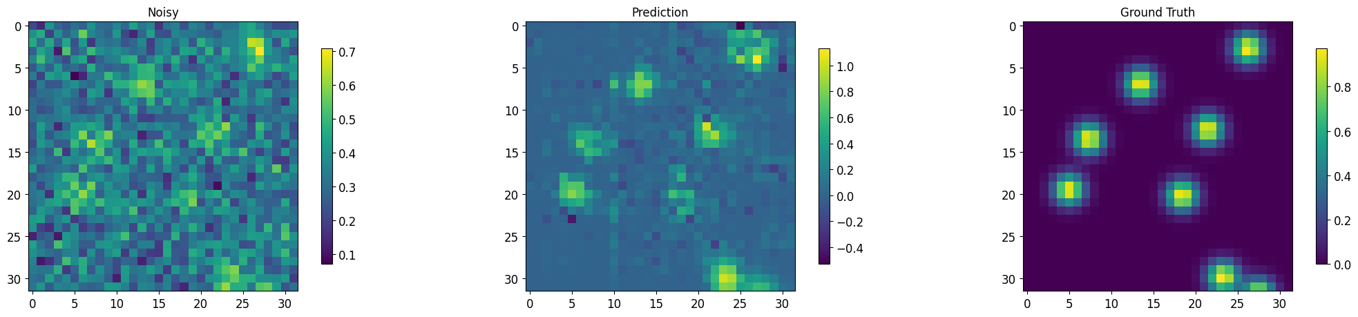
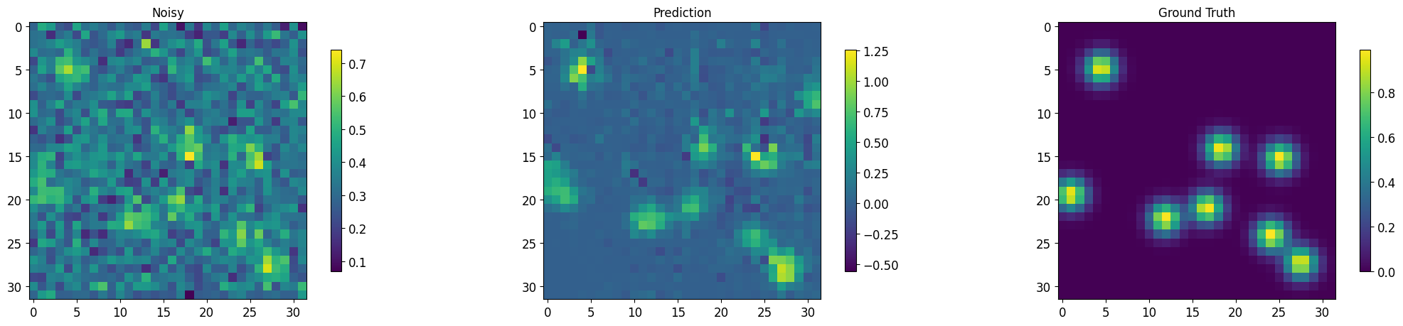
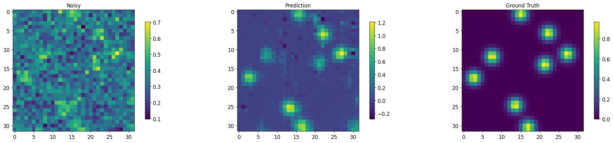
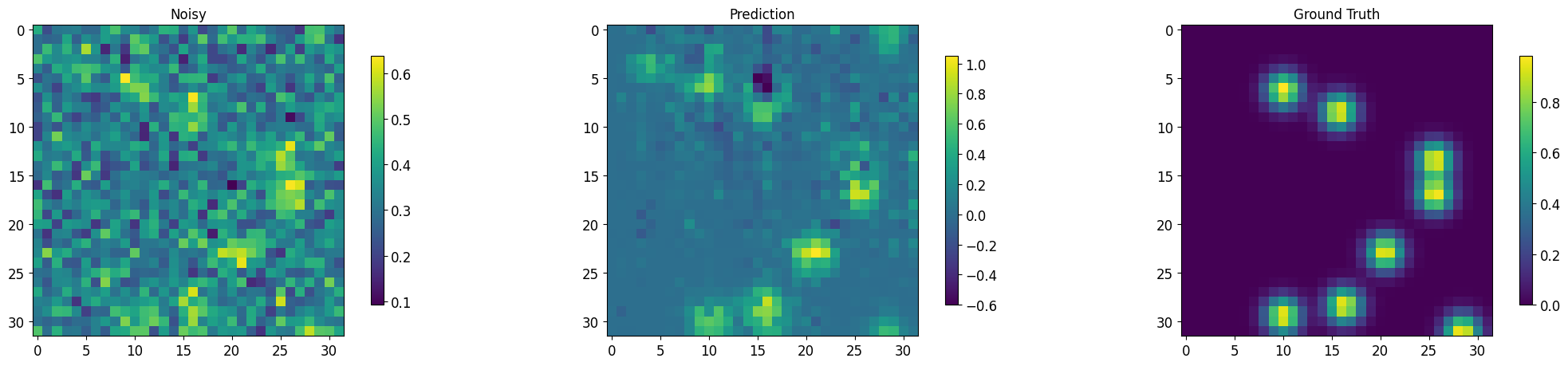
MSDNet predictions

output, noisy, target  = segment_imgs(test_loader, msdnet_model, num_display=3)

Images for batch # 1, number 0

Images for batch # 1, number 1

Images for batch # 1, number 2

Images for batch # 1, number 3

Images for batch # 1, number 4

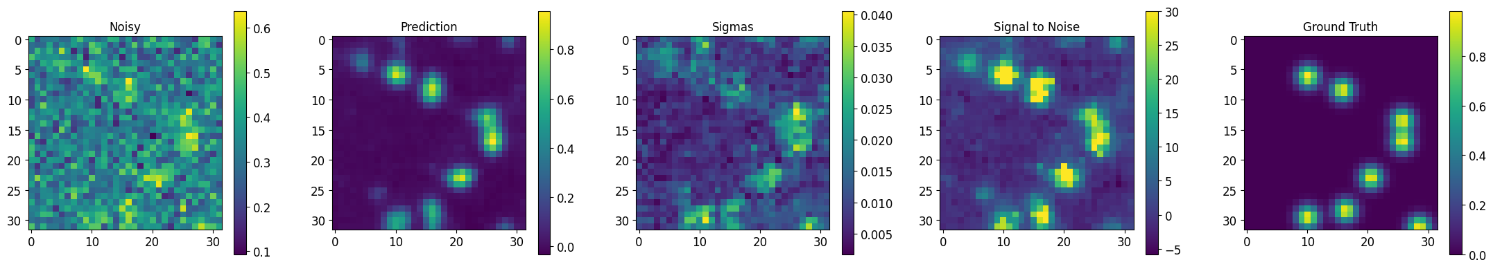
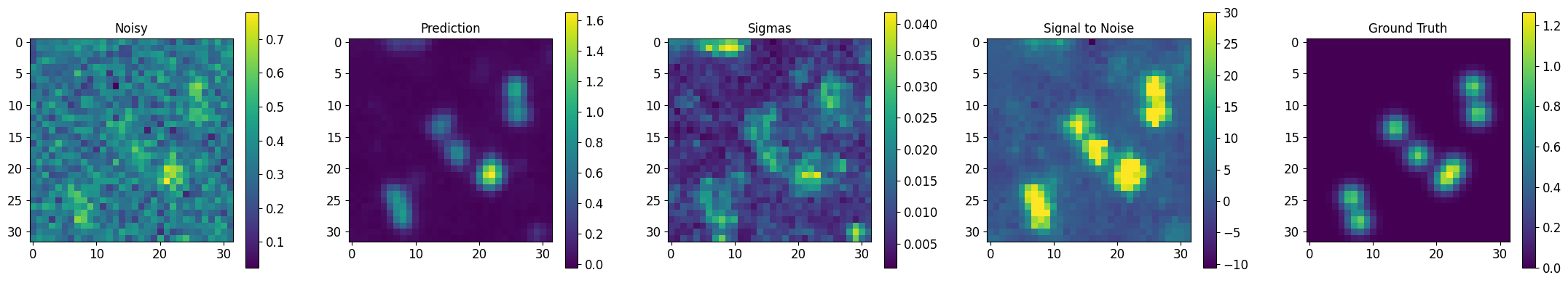
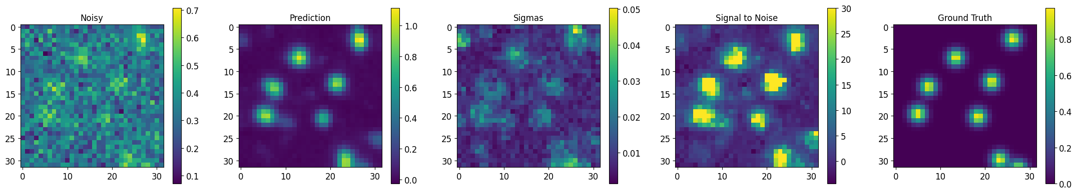
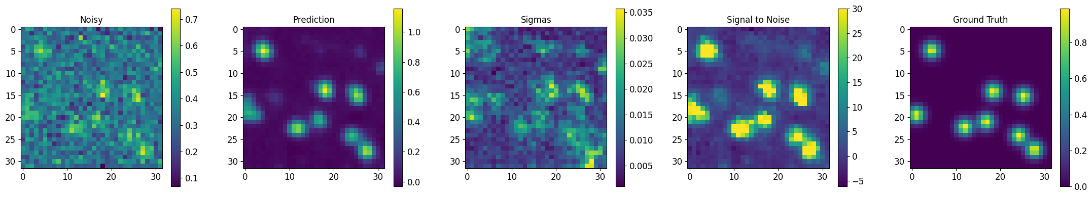
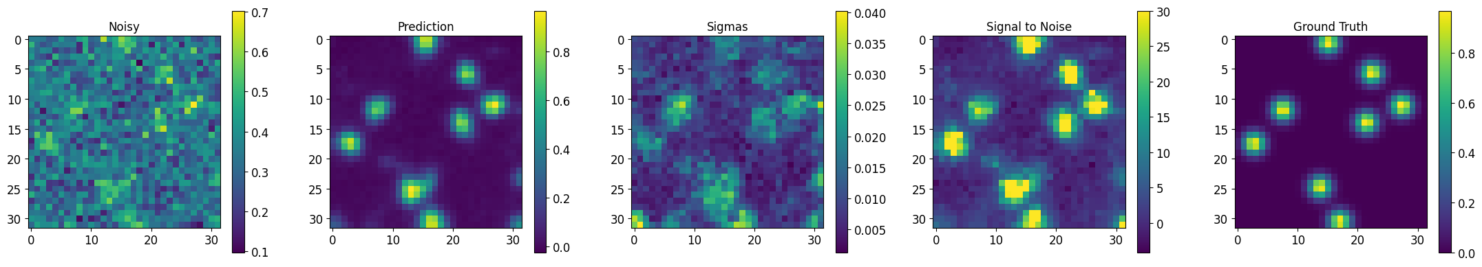
RMSNet predictions

The multiple RMSNets are ‘ensembled’ together using bagging. Displayed here are:

• Noisy/Prediction: original noisy images and denoised network ensemble predictions,

• Sigmas: standard deviation of denoising predictions

• Signal to Noise: Prediction / Sigmas

bagged_model = baggins.model_baggin(nets,"regression", False)

output, noisy, target  = segment_imgs(test_loader, bagged_model, std=True)

Images for batch # 1, number 0

Images for batch # 1, number 1

Images for batch # 1, number 2

Images for batch # 1, number 3

Images for batch # 1, number 4