Latent Space Exploration with UMap and Randomized Sparse Mixed Scale Autoencoders
Authors: Eric Roberts and Petrus Zwart
E-mail: PHZwart@lbl.gov, EJRoberts@lbl.gov
This notebook highlights some basic functionality with the dlsia package.
We will setup randomly connected, sparse mixed-scale inspired autoencoders with for unsupervised learning, with the goal of exploring the latent space it generates. These autoencoders deploy random sparsely connected convolutions and random downsampling/upsampling operations (maxpooling/transposed convolutions) for compressing/expanding data in the encoder/decoder halves. This random layout supplants the structured order of typical Autoencoders, which consist downsampling/upsampling operations following dual convolutions.
Like the preceding sparse mixed-scale networks (SMSNets), there exist a number of hyperparameters to tweak so we can control the number of learnable parameters these sparsely connected networks contain. This type of control can be beneficial when the amount of data on which one can train a network is not very voluminous, as it allows for better handles on overfitting.
[1]:
import numpy as np

import torch
import torch.nn as nn
import torch.optim as optim

from dlsia.core import helpers
from dlsia.core import train_scripts
from dlsia.core.networks import sparsenet
from dlsia.test_data.two_d import random_shapes
from dlsia.core.utils import latent_space_viewer
from dlsia.viz_tools import plots, draw_sparse_network

import matplotlib.pyplot as plt
from torch.utils.data import DataLoader, TensorDataset
import einops
import umap

from IPython.display import Image
Create Data
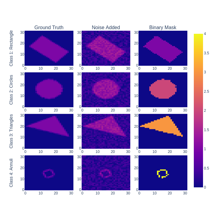
Using our dlsia in-house data generator, we produce a number of noisy “shapes” images consisting of single triangles, rectangles, circles, and donuts/annuli, each assigned a different class. In addition to augmenting with random orientations and sizes, each raw, ground truth image will be bundled with its corresponding noisy and binary mask.
Parameters to toggle:
n_train : number of ground truth/noisy/label image bundles to generate for training
n_test : number of ground truth/noisy/label image bundles to generate for testing
noise_level : per-pixel noise drawn from a continuous uniform distribution (cut-off above at 1)
N_xy : size of individual images
[2]:
N_train = 500
N_test  = 15000
noise_level = 0.50
Nxy = 32

train_data = random_shapes.build_random_shape_set_numpy(n_imgs=N_train,
                                                        noise_level=noise_level,
                                                        n_xy=Nxy)
test_data = random_shapes.build_random_shape_set_numpy(n_imgs=N_test,
                                                       noise_level=noise_level,
                                                       n_xy=Nxy)

test_GT = torch.Tensor(test_data["GroundTruth"]).unsqueeze(1)
View shapes data
[3]:
# normally we would use interactive plot here via
# plots.plot_shapes_data_numpy(train_data).show()
# but they don't survive when displayed in github, so
# we make it a static plot instead.
tmp = plots.plot_shapes_data_numpy(train_data)
tmp = tmp.to_image(format="png", scale=1.0)
Image(tmp)
[3]:
Dataloader class
Here we cast all images from numpy arrays and the PyTorch Dataloader class for easy handling and iterative loading of data into the networks and models.
[4]:
which_one = "Noisy" #"GroundTruth"

batch_size = 100

loader_params = {'batch_size': batch_size,
                 'shuffle': True}
Ttrain_data = TensorDataset( torch.Tensor(train_data[which_one]).unsqueeze(1) )

train_loader = DataLoader(Ttrain_data, **loader_params)

loader_params = {'batch_size': batch_size,
                 'shuffle': False}
test_data = TensorDataset( torch.Tensor(test_data[which_one][0:N_train]).unsqueeze(1) )
test_loader = DataLoader(test_data, **loader_params)

demo_data = TensorDataset( torch.Tensor(test_data[which_one]).unsqueeze(1) )
demo_loader = DataLoader(demo_data, **loader_params)
Build Autoencoder
There are a number of parameters to play with that impact the size of the network:
Hyperparameters to toggle
latent_shape: the spatial footprint of the image in latent space. I don’t recommend going below 4x4, because it interferes with the dilation choices. This is a bit of a bug, we need to fix that. Its on the list.
out_channels: the number of channels of the latent image. Determines the dimension of latent space: (channels,latent_shape[-2], latent_shape[-1])
depth: the depth of the random sparse convolutional encoder / decoder
hidden channels: The number of channels put out per convolution.
max_degree / min_degree : This determines how many connections you have per node.
Other parameters do not impact the size of the network dramatically / at all:
in_shape: determined by the input shape of the image.
dilations: the maximum dilation should not exceed the smallest image dimension.
alpha_range: determines the type of graphs (wide vs skinny). When alpha is large,the chances for skinny graphs to be generated increases. We don’t know which parameter choice is best, so we randomize it’s choice.
gamma_range: no effect unless the maximum degree and min_degree are far apart. We don’t know which parameter choice is best, so we randomize it’s choice.
pIL, pLO, IO: keep as is.
stride_base: make sure your latent image size can be generated from the in_shape by repeated division of with this number.
[5]:
autoencoder = sparsenet.SparseAutoEncoder(in_shape=(32, 32),
                                          latent_shape=(4, 4),
                                          depth=20,
                                          dilations=[1,2,3],
                                          hidden_channels=4,
                                          out_channels=1,
                                          alpha_range=(0.05, 0.25),
                                          gamma_range=(0.0, 0.5),
                                          max_degree=10, min_degree=4,
                                          pIL=0.15,
                                          pLO=0.15,
                                          IO=False,
                                          stride_base=2)
pytorch_total_params = helpers.count_parameters(autoencoder)
print( "Number of parameters:", pytorch_total_params)
Number of parameters: 82798
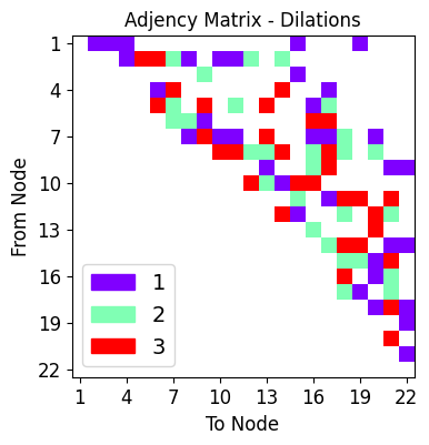
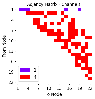
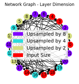
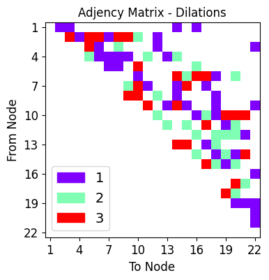
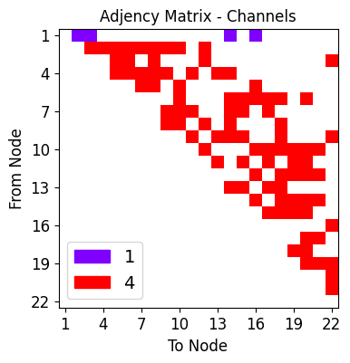
Visualize encoder half
We visualize the layout of connections in the encoder half of the Autoencoder, the first half responsible for the lower-dimensional compression of the data in the latent space.
[6]:
ne,de,ce = draw_sparse_network.draw_network(autoencoder.encode)

Visualize decoder half
Now the visualization of connections comprising the decoder half of the Autoencoder. This second half is responsible for reconstructing the exact image input from the compressed information in the latent space
[7]:
nd,dd,cd = draw_sparse_network.draw_network(autoencoder.decode)
Training the Autoencoder
Training hyperparameters are specified.
[8]:
device = helpers.get_device()

learning_rate = 1e-3
num_epochs=50
criterion = nn.L1Loss()
optimizer = optim.Adam(autoencoder.parameters(), lr=learning_rate)
Training loop
[9]:
rv = train_scripts.train_autoencoder(net=autoencoder.to(device),
                                     trainloader=train_loader,
                                     validationloader=test_loader,
                                     NUM_EPOCHS=num_epochs,
                                     criterion=criterion,
                                     optimizer=optimizer,
                                     device=device,
                                     show=10)
print("Best Performance:", rv[1]["CC validation"][rv[1]['Best model index']])
Epoch 10 of 50 | Learning rate 1.000e-03
Training Loss: 2.1247e-01 | Validation Loss: 2.0973e-01
Training CC: 0.6644   Validation CC  : 0.6795
Epoch 20 of 50 | Learning rate 1.000e-03
Training Loss: 1.7950e-01 | Validation Loss: 1.8015e-01
Training CC: 0.7929   Validation CC  : 0.7947
Epoch 30 of 50 | Learning rate 1.000e-03
Training Loss: 1.6541e-01 | Validation Loss: 1.6835e-01
Training CC: 0.8358   Validation CC  : 0.8309
Epoch 40 of 50 | Learning rate 1.000e-03
Training Loss: 1.5865e-01 | Validation Loss: 1.6228e-01
Training CC: 0.8541   Validation CC  : 0.8474
Epoch 50 of 50 | Learning rate 1.000e-03
Training Loss: 1.5353e-01 | Validation Loss: 1.5887e-01
Training CC: 0.8657   Validation CC  : 0.8560
Best Performance: 0.8560476422309875
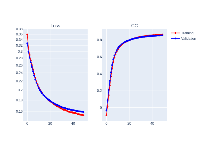
[10]:
# normally we would use interactive plot here,
# but they don't survive when displayed in github, so
# we make it a static plot instead.

tmp = plots.plot_training_results_regression(rv[1])
tmp = tmp.to_image(format="png", scale=1.0)
Image(tmp)
[10]:
Latent space exploration
With the full SMSNet-Autoencoder trained, we pass new testing data through the encoder-half and apply Uniform Manifold Approximation and Projection (UMap), a nonlinear dimensionality reduction technique leveraging topological structures.
Visualize raw latent space
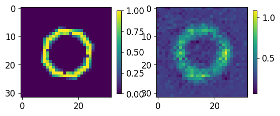
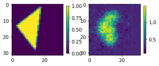
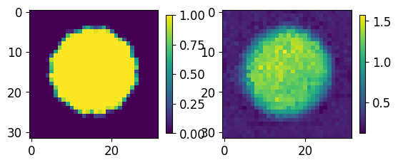
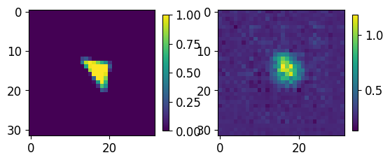
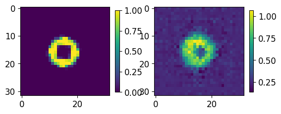
Test images previously unseen by the network are shown in their latent space representation.
[11]:
results = []
latent = []
for batch in demo_loader:
    with torch.no_grad():
        res = autoencoder(batch[0].to(device))
        lt = autoencoder.latent_vector(batch[0].to(device))
        results.append(res.cpu())
        latent.append(lt.cpu())
results = torch.cat(results, dim=0)
latent = torch.cat(latent, dim=0)
[12]:
for ii,jj in zip(test_GT.numpy()[0:5],results.numpy()[0:5]):
    fig, axs = plt.subplots(1,2)
    im00 = axs[0].imshow(ii[0,...])
    im01 = axs[1].imshow(jj[0])
    plt.colorbar(im00,ax=axs[0], shrink=0.45)
    plt.colorbar(im01,ax=axs[1], shrink=0.45)
    plt.show()
    print("-----------------")
-----------------
-----------------
-----------------
-----------------
-----------------
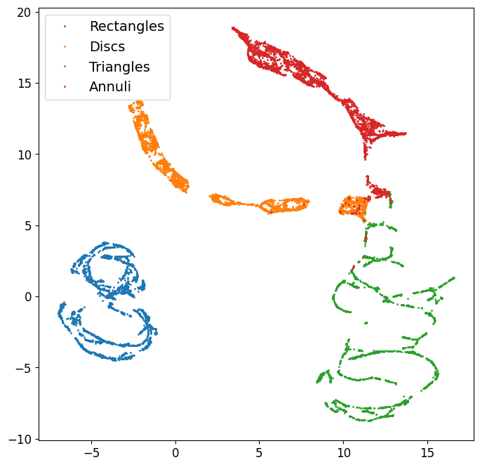
UMap compression
Autoencoder latent space is further reduced down to two dimensions; i.e. each image passed though the encoder is represented by an integer pair of coordinates below, with blue repesenting all rectangles, orange representing all circles/discs, green representing all triangles, and red representing all annuli.
UMap parameters
We outline below a few key parameters. (Further investigation into UMap capabilities can be found on UMap documentation page.)
min_dist: controls how tightly points may be packed together (default is 0.1).
n_neighbors: controls balance of local vs. global structure in the data (default is 15).
n_components: dimensionality of final reduction (default is 2; for 3d embedding, use n_components=3).
[13]:
umapper = umap.UMAP(min_dist=0, n_neighbors=35)
X = umapper.fit_transform(latent.numpy())
[14]:
these_labels = test_data["Label"]
plt.figure(figsize=(8,8))
for lbl in [1,2,3,4]:
    sel = these_labels==lbl
    plt.plot(X[sel,0], X[sel,1], '.', markersize=2)
plt.legend(["Rectangles","Discs","Triangles","Annuli"])
plt.show()
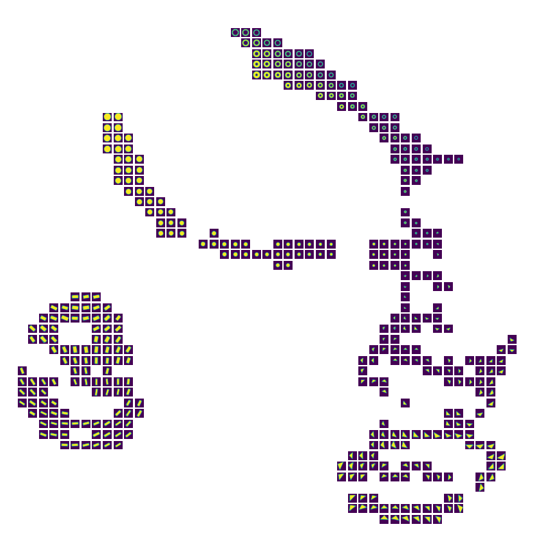
Below simply averages all nearest-neighbors for visualization purposed.
[15]:
fig = latent_space_viewer.build_latent_space_image_viewer(test_data["GroundTruth"],
                                                          X,
                                                          n_bins=50,
                                                          min_count=1,
                                                          max_count=1,
                                                          mode="mean"
                                                         )
[ ]: