Image classification via an ensemble of Randomized Sparse Mixed Scale Networks

Authors: Eric Roberts and Petrus Zwart

E-mail: PHZwart@lbl.gov, EJRoberts@lbl.gov

This notebook highlights some basic functionality with the dlsia package.

In this notebook we will demonstrate an ensemble method for image classification. We define a few randomized sparse mixed scale networks (RMSNets), then append fully connected layers to yield an image classifier. We will train a few independent networks that will be combined into a single classifier that yields both a probability and associated standard deviation.

import numpy as np

import torch
import torch.nn as nn
import torch.optim as optim

from dlsia.core import helpers
from dlsia.core import train_scripts
from dlsia.core.networks import sparsenet
from dlsia.core.networks import baggins
from dlsia.test_data.two_d import random_shapes
from dlsia.core.utils import latent_space_viewer
from dlsia.viz_tools import plots
from dlsia.viz_tools import plot_autoencoder_image_classification as paic


import matplotlib.pyplot as plt
from torch.utils.data import DataLoader, TensorDataset
import einops
import umap

from IPython.display import Image

Create data

Using our dlsia in-house data generator, we produce a number of noisy “shapes” images consisting of single triangles, rectangles, circles, and donuts/annuli, each assigned a different class. In addition to augmenting with random orientations and sizes, each raw, ground truth image will be bundled with its corresponding noisy and binary mask.

Parameters to toggle:

• N_train : number of ground truth/noisy/label image bundles to generate for training

• N_labeled : number of images with labels

• N_test : number of ground truth/noisy/label image bundles to generate for testing

• noise_level : per-pixel noise drawn from a continuous uniform distribution (cut-off above at 1)

• Nxy : size of individual images

N_train = 100
N_labeled = 100

N_test  = 5000
noise_level = 0.005
Nxy = 32

train_data = random_shapes.build_random_shape_set_numpy(n_imgs=N_train,
                                                        noise_level=noise_level,
                                                        n_xy=Nxy)
test_data = random_shapes.build_random_shape_set_numpy(n_imgs=N_test,
                                                       noise_level=noise_level,
                                                       n_xy=Nxy)

View shapes data

plots.plot_shapes_data_numpy(train_data)

Dataloader class

Here we cast all images from numpy arrays and the PyTorch Dataloader class for easy handling and iterative loading of data into the networks and models.

Once again, to reduce/increase memory consumption, tune the batch_size parameter.

which_one = "Noisy"

batch_size = 100

loader_params = {'batch_size': batch_size,
                 'shuffle': True}
train_imgs = torch.Tensor(train_data[which_one]).unsqueeze(1)
train_labels = torch.Tensor(train_data["Label"]).unsqueeze(1)-1
train_labels[N_labeled:]=-1 # remove some labels to highlight 'mixed' training

train_data = TensorDataset(train_imgs,train_labels)
train_loader = DataLoader(train_data, **loader_params)

loader_params = {'batch_size': batch_size,
                 'shuffle': False}
test_images = torch.Tensor(test_data[which_one]).unsqueeze(1)
test_labels = torch.Tensor(test_data["Label"]).unsqueeze(1)-1
test_data = TensorDataset(test_images, test_labels )
test_loader = DataLoader(test_data, **loader_params)

Build SMSNets

Define SMSNet (Sparse Mixed-Scale Network) architecture-governing hyperparameters here.

Lets build some neural networks

Hyperparameters to toggle

There are a number of parameters to play with that impact the size of the network:

• latent_shape: the spatial footprint of the image in latent space. I don’t recommend going below 4x4, because it interferes with the dilation choices. This is a bit of a annoying feature, we need to fix that. It’s on the list.

• out_channels: the number of channels of the latent image. Determines the dimension of latent space: (channels,latent_shape[-2], latent_shape[-1])

• depth: the depth of the random sparse convolutional encoder.

• hidden channels: The number of channels put out per convolution.

• max_degree / min_degree : This determines how many connections you have per node.

Other parameters do not impact the size of the network dramatically / at all:

• in_shape: determined by the input shape of the image.

• dilations: the maximum dilation should not exceed the smallest image dimension.

• alpha_range: determines the type of graphs (wide vs skinny). When alpha is large, the chances for skinny graphs to be generated increases. We don’t know which parameter choice is best, so we randomize it’s choice.

• gamma_range: no effect unless the maximum degree and min_degree are far apart. We don’t know which parameter choice is best, so we randomize it’s choice.

• pIL,pLO,IO: keep as is.

• stride_base: make sure your latent image size can be generated from the in_shape by repeated division of with this number.

For the classification, specify the number of output classes. Here we work with 4 shapes, so set it to 4. The dropout rate governs the dropout layers in the classifier part of the networks and doesn’t affect the encoder part.

Initialize the networks

networks = []
Nmodels = 3
for ii in range(Nmodels):
    rando = sparsenet.SparseLabeler(in_shape=(32, 32),
                                    latent_shape=(8, 8),
                                    out_classes=4,
                                    depth=10,
                                    dilations=[1,2,3,4],
                                    hidden_channels=3,
                                    in_channels=1,
                                    out_channels=1,
                                    alpha_range=(0.75, 1.0),
                                    gamma_range=(0.0, 0.5),
                                    max_degree=4, min_degree=2,
                                    pIL=0.15,
                                    pLO=0.15,
                                    IO=False,
                                    stride_base=2,
                                    dropout_rate=0.15
                                   )
    networks.append(rando)
    pytorch_total_params = helpers.count_parameters(rando)
    print( "Number of parameters in network", ii , ': ', pytorch_total_params)

Number of parameters in network 0 :  7791
Number of parameters in network 1 :  8124
Number of parameters in network 2 :  6930

Train networks

We specify the learning rate and the number of epochs for used for each training instance.

Note: we define two optimizers: one for autoencoding and one for classification. They will be minimized in sequence (one after another) instead of building a single sum of targets. This avoids choosing the right weight.

The mini-epochs are the number of epochs it passes over the whole data set to optimize a single target function. The autoencoder is done first.

learning_rate = 1e-3
num_epochs=25
device = helpers.get_device()
F1_scores = []

for ii in range(Nmodels):
    print('Network: ', ii)
    rando = networks[ii]
    torch.cuda.empty_cache()

    criterion_label = nn.CrossEntropyLoss()
    optimizer_label = optim.Adam(rando.parameters(), lr=learning_rate)

    rv = train_scripts.train_labeling(net=rando.to(device),
                                      trainloader=train_loader,
                                      validationloader=test_loader,
                                      NUM_EPOCHS=num_epochs,
                                      criterion=criterion_label,
                                      optimizer=optimizer_label,
                                      device=device,
                                      show=25,
                                      clip_value=100.0)
    #plots.plot_training_results_segmentation(rv[1]).show()
    F1_scores.append(rv[1]['F1 validation macro'][rv[1]['Best model index']])

Network:  0
Epoch 25 of 25 | Learning rate 1.000e-03
   Training Loss: 5.1590e-01 | Validation Loss: 8.6460e-01
   Micro Training F1: 0.8600 | Micro Validation F1: 0.6364
   Macro Training F1: 0.8611 | Macro Validation F1: 0.6318
Network:  1
Epoch 25 of 25 | Learning rate 1.000e-03
   Training Loss: 6.0787e-01 | Validation Loss: 1.0655e+00
   Micro Training F1: 0.8100 | Micro Validation F1: 0.5382
   Macro Training F1: 0.8012 | Macro Validation F1: 0.5357
Network:  2
Epoch 25 of 25 | Learning rate 1.000e-03
   Training Loss: 7.2811e-01 | Validation Loss: 1.0883e+00
   Micro Training F1: 0.7500 | Micro Validation F1: 0.5218
   Macro Training F1: 0.7641 | Macro Validation F1: 0.5236

Network evaluation

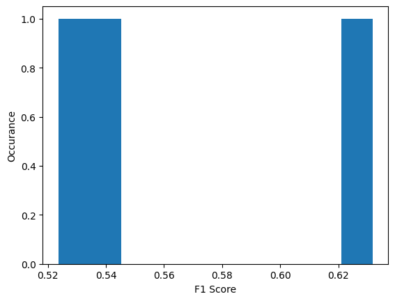
F1 score distribution

The individual models performances are far from ideal. When we make an ensemble model things will look a lot better.

plt.hist(F1_scores, bins=10)
plt.xlabel("F1 Score")
plt.ylabel("Occurance")
plt.show()

Bagging networks

bagged_model = baggins.model_baggin(networks)

Lets go over the full validation dataset and see what we get

mean = []
std = []
true_lbl = []
inp_img = []
inferred_label = []
for batch in test_loader:
    true_lbl.append(batch[1])
    with torch.no_grad():
        inp_img.append(batch[0].cpu())
        mp,sp = bagged_model(batch[0], device, True)
        mean.append(mp.cpu())
        std.append(sp.cpu())
        guessed = torch.argmax(mp, axis=-1)
        inferred_label.append(guessed)
mean = torch.cat(mean, dim=0)
std = torch.cat(std, dim=0)
true_lbl = torch.cat(true_lbl, dim=0)
inp_img = torch.cat(inp_img, dim=0)
inferred_label = torch.cat(inferred_label, dim=0).unsqueeze(-1)

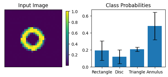
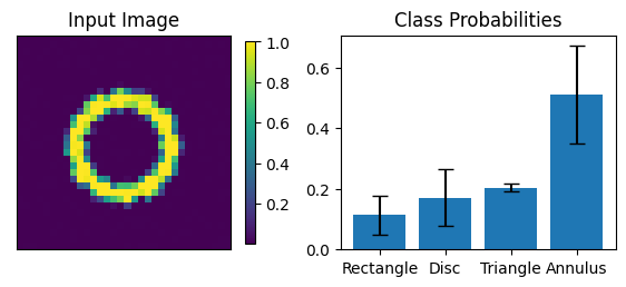
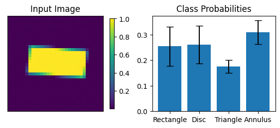
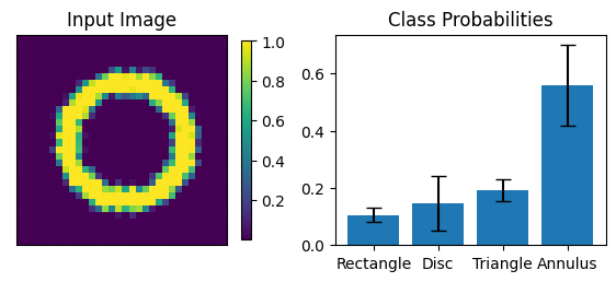
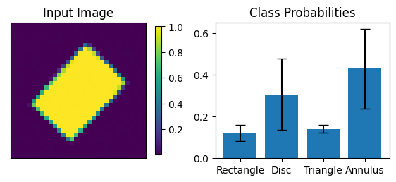
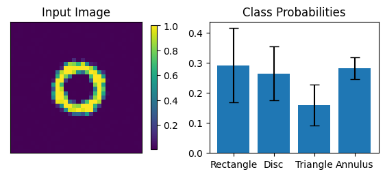
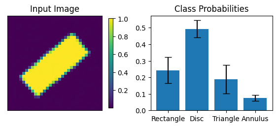
View predictions

We compute F1 metrics and visualize the image classification results.

count=0
tmp = train_scripts.segmentation_metrics(mean,
                                         true_lbl.flatten().type(torch.LongTensor),
                                         missing_label=-1)
print(f"Macro F1 on Test Data {tmp[0]: 6.5f}")
print(f"Micro F1 on Test Data {tmp[1]: 6.5f}")
print()
assert tmp[1] > 0.75 # just to make sure all is ok

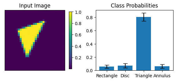
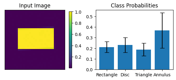
print("--------       The first 5 images encountered     ----------")
for mp,sp,tlbl,ilbl,img in zip(mean, std, true_lbl.flatten(), inferred_label.flatten(), inp_img):
    fig = paic.plot_image_and_class_probabilities(input_img=img[0].numpy(),
                                       class_names= ["Rectangle","Disc","Triangle","Annulus"],
                                       p_classification=mp.numpy(),
                                       std_p_classification=sp.numpy())
    plt.show()
    count += 1
    if count > 5:
        break
print()
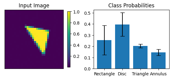
print("--------       Incorrectly classified images (5 maximum)   ----------")
count=0
for mp,sp,tlbl,ilbl,img in zip(mean, std, true_lbl.flatten(), inferred_label.flatten(), inp_img):
    if int(tlbl) != int(ilbl):
        fig = paic.plot_image_and_class_probabilities(input_img=img[0].numpy(),
                                           class_names= ["Rectangle","Disc","Triangle","Annulus"],
                                           p_classification=mp.numpy(),
                                           std_p_classification=sp.numpy())
        count += 1
        if count > 5:
            break

Macro F1 on Test Data  0.75540
Micro F1 on Test Data  0.75380

--------       The first 5 images encountered     ----------

--------       Incorrectly classified images (5 maximum)   ----------

Notes on saving random networks

It would be nice to save these networks of course. The issue is that the networks are generated using a random number generator, and have no predetermined topology. Because of this feature, some utility functions have been developed.

Saving a random network is done via its “save_network_parameters” function. If a file name is supplied, a small file will be saved, if the filename is not supplied, an OrderedDict will be returned. A saved network parameter file can be used to instantiate that same network via the SparseLabeler_from_file method.

import os

savepath = 'ensembleNetworks'
if os.path.exists(savepath) is False:
    os.mkdir(savepath)

new_networks = []
for ii in range(Nmodels):
    name = savepath + "/model_%i.pt"%ii
    networks[ii].save_network_parameters(name)
    new_networks.append(sparsenet.SparseLabeler_from_file(name))